case study hypothesis testing

User Preferences

Content preview.

Arcu felis bibendum ut tristique et egestas quis:

• Ut enim ad minim veniam, quis nostrud exercitation ullamco laboris
• Duis aute irure dolor in reprehenderit in voluptate
• Excepteur sint occaecat cupidatat non proident

Keyboard Shortcuts

S.3 hypothesis testing.

In reviewing hypothesis tests, we start first with the general idea. Then, we keep returning to the basic procedures of hypothesis testing, each time adding a little more detail.

The general idea of hypothesis testing involves:

• Making an initial assumption.
• Collecting evidence (data).
• Based on the available evidence (data), deciding whether to reject or not reject the initial assumption.

Every hypothesis test — regardless of the population parameter involved — requires the above three steps.

Example S.3.1

Is normal body temperature really 98.6 degrees f section  .

Consider the population of many, many adults. A researcher hypothesized that the average adult body temperature is lower than the often-advertised 98.6 degrees F. That is, the researcher wants an answer to the question: "Is the average adult body temperature 98.6 degrees? Or is it lower?" To answer his research question, the researcher starts by assuming that the average adult body temperature was 98.6 degrees F.

Then, the researcher went out and tried to find evidence that refutes his initial assumption. In doing so, he selects a random sample of 130 adults. The average body temperature of the 130 sampled adults is 98.25 degrees.

Then, the researcher uses the data he collected to make a decision about his initial assumption. It is either likely or unlikely that the researcher would collect the evidence he did given his initial assumption that the average adult body temperature is 98.6 degrees:

• If it is likely , then the researcher does not reject his initial assumption that the average adult body temperature is 98.6 degrees. There is not enough evidence to do otherwise.
• either the researcher's initial assumption is correct and he experienced a very unusual event;
• or the researcher's initial assumption is incorrect.

In statistics, we generally don't make claims that require us to believe that a very unusual event happened. That is, in the practice of statistics, if the evidence (data) we collected is unlikely in light of the initial assumption, then we reject our initial assumption.

Example S.3.2

Criminal trial analogy section  .

One place where you can consistently see the general idea of hypothesis testing in action is in criminal trials held in the United States. Our criminal justice system assumes "the defendant is innocent until proven guilty." That is, our initial assumption is that the defendant is innocent.

In the practice of statistics, we make our initial assumption when we state our two competing hypotheses -- the null hypothesis ( H 0 ) and the alternative hypothesis ( H A ). Here, our hypotheses are:

• H 0 : Defendant is not guilty (innocent)
• H A : Defendant is guilty

In statistics, we always assume the null hypothesis is true . That is, the null hypothesis is always our initial assumption.

The prosecution team then collects evidence — such as finger prints, blood spots, hair samples, carpet fibers, shoe prints, ransom notes, and handwriting samples — with the hopes of finding "sufficient evidence" to make the assumption of innocence refutable.

In statistics, the data are the evidence.

The jury then makes a decision based on the available evidence:

• If the jury finds sufficient evidence — beyond a reasonable doubt — to make the assumption of innocence refutable, the jury rejects the null hypothesis and deems the defendant guilty. We behave as if the defendant is guilty.
• If there is insufficient evidence, then the jury does not reject the null hypothesis . We behave as if the defendant is innocent.

In statistics, we always make one of two decisions. We either "reject the null hypothesis" or we "fail to reject the null hypothesis."

Errors in Hypothesis Testing Section  

Did you notice the use of the phrase "behave as if" in the previous discussion? We "behave as if" the defendant is guilty; we do not "prove" that the defendant is guilty. And, we "behave as if" the defendant is innocent; we do not "prove" that the defendant is innocent.

This is a very important distinction! We make our decision based on evidence not on 100% guaranteed proof. Again:

• If we reject the null hypothesis, we do not prove that the alternative hypothesis is true.
• If we do not reject the null hypothesis, we do not prove that the null hypothesis is true.

We merely state that there is enough evidence to behave one way or the other. This is always true in statistics! Because of this, whatever the decision, there is always a chance that we made an error .

Let's review the two types of errors that can be made in criminal trials:

Table S.3.2 shows how this corresponds to the two types of errors in hypothesis testing.

Note that, in statistics, we call the two types of errors by two different  names -- one is called a "Type I error," and the other is called  a "Type II error." Here are the formal definitions of the two types of errors:

There is always a chance of making one of these errors. But, a good scientific study will minimize the chance of doing so!

Making the Decision Section  

Recall that it is either likely or unlikely that we would observe the evidence we did given our initial assumption. If it is likely , we do not reject the null hypothesis. If it is unlikely , then we reject the null hypothesis in favor of the alternative hypothesis. Effectively, then, making the decision reduces to determining "likely" or "unlikely."

In statistics, there are two ways to determine whether the evidence is likely or unlikely given the initial assumption:

• We could take the " critical value approach " (favored in many of the older textbooks).
• Or, we could take the " P -value approach " (what is used most often in research, journal articles, and statistical software).

In the next two sections, we review the procedures behind each of these two approaches. To make our review concrete, let's imagine that μ is the average grade point average of all American students who major in mathematics. We first review the critical value approach for conducting each of the following three hypothesis tests about the population mean $\mu$:

In Practice

• We would want to conduct the first hypothesis test if we were interested in concluding that the average grade point average of the group is more than 3.
• We would want to conduct the second hypothesis test if we were interested in concluding that the average grade point average of the group is less than 3.
• And, we would want to conduct the third hypothesis test if we were only interested in concluding that the average grade point average of the group differs from 3 (without caring whether it is more or less than 3).

Upon completing the review of the critical value approach, we review the P -value approach for conducting each of the above three hypothesis tests about the population mean \(\mu\). The procedures that we review here for both approaches easily extend to hypothesis tests about any other population parameter.

All Courses

• Interview Questions
• Free Courses
• Career Guide
• PGP in Data Science and Business Analytics
• PG Program in Data Science and Business Analytics Classroom
• PGP in Data Science and Engineering (Data Science Specialization)
• PGP in Data Science and Engineering (Bootcamp)
• PGP in Data Science & Engineering (Data Engineering Specialization)
• Master of Data Science (Global) – Deakin University
• MIT Data Science and Machine Learning Course Online
• Master’s (MS) in Data Science Online Degree Programme
• MTech in Data Science & Machine Learning by PES University
• Data Analytics Essentials by UT Austin
• Data Science & Business Analytics Program by McCombs School of Business
• MTech In Big Data Analytics by SRM
• M.Tech in Data Engineering Specialization by SRM University
• M.Tech in Big Data Analytics by SRM University
• PG in AI & Machine Learning Course
• Weekend Classroom PG Program For AI & ML
• AI for Leaders & Managers (PG Certificate Course)
• Artificial Intelligence Course for School Students
• IIIT Delhi: PG Diploma in Artificial Intelligence
• Machine Learning PG Program
• MIT No-Code AI and Machine Learning Course
• Study Abroad: Masters Programs
• MS in Information Science: Machine Learning From University of Arizon
• SRM M Tech in AI and ML for Working Professionals Program
• UT Austin Artificial Intelligence (AI) for Leaders & Managers
• UT Austin Artificial Intelligence and Machine Learning Program Online
• MS in Machine Learning
• IIT Roorkee Full Stack Developer Course
• IIT Madras Blockchain Course (Online Software Engineering)
• IIIT Hyderabad Software Engg for Data Science Course (Comprehensive)
• IIIT Hyderabad Software Engg for Data Science Course (Accelerated)
• IIT Bombay UX Design Course – Online PG Certificate Program
• Online MCA Degree Course by JAIN (Deemed-to-be University)
• Cybersecurity PG Course
• Online Post Graduate Executive Management Program
• Product Management Course Online in India
• NUS Future Leadership Program for Business Managers and Leaders
• PES Executive MBA Degree Program for Working Professionals
• Online BBA Degree Course by JAIN (Deemed-to-be University)
• MBA in Digital Marketing or Data Science by JAIN (Deemed-to-be University)
• Master of Business Administration- Shiva Nadar University
• Post Graduate Diploma in Management (Online) by Great Lakes
• Online MBA Programs
• Cloud Computing PG Program by Great Lakes
• University Programs
• Stanford Design Thinking Course Online
• Design Thinking : From Insights to Viability
• PGP In Strategic Digital Marketing
• Post Graduate Diploma in Management
• Master of Business Administration Degree Program
• MS in Business Analytics in USA
• MS in Machine Learning in USA
• Study MBA in Germany at FOM University
• M.Sc in Big Data & Business Analytics in Germany
• Study MBA in USA at Walsh College
• MS Data Analytics
• MS Artificial Intelligence and Machine Learning
• MS in Data Analytics
• Master of Business Administration (MBA)
• MS in Information Science: Machine Learning
• MS in Machine Learning Online
• MIT Data Science Program
• AI For Leaders Course
• Data Science and Business Analytics Course
• Cyber Security Course
• PG Program Online Artificial Intelligence Machine Learning
• PG Program Online Cloud Computing Course
• Data Analytics Essentials Online Course
• MIT Programa Ciencia De Dados Machine Learning
• MIT Programa Ciencia De Datos Aprendizaje Automatico
• Program PG Ciencia Datos Analitica Empresarial Curso Online
• Mit Programa Ciencia De Datos Aprendizaje Automatico
• Online Data Science Business Analytics Course
• Online Ai Machine Learning Course
• Online Full Stack Software Development Course
• Online Cloud Computing Course
• Cybersecurity Course Online
• Online Data Analytics Essentials Course
• Ai for Business Leaders Course
• Mit Data Science Program
• No Code Artificial Intelligence Machine Learning Program
• MS Information Science Machine Learning University Arizona
• Wharton Online Advanced Digital Marketing Program
• Introduction to Hypothesis Testing in R
• Testing of Hypothesis in R
• p-value: An Alternative way of Hypothesis Testing:
• t-test: Hypothesis Testing of Population Mean when Population Standard Deviation is Unknown:
• Two Samples Tests: Hypothesis Testing for the difference between two population means
• Hypothesis Testing for Equality of Population Variances
• Let’s Look at some Case studies:
• References:

Hypothesis Testing in R- Introduction Examples and Case Study

– By Dr. Masood H. Siddiqui, Professor & Dean (Research) at Jaipuria Institute of Management, Lucknow

The premise of Data Analytics is based on the philosophy of the “ Data-Driven Decision Making ” that univocally states that decision-making based on data has less probability of error than those based on subjective judgement and gut-feeling. So, we require data to make decisions and to answer the business/functional questions. Data may be collected from each and every unit/person, connected with the problem-situation (totality related to the situation). This is known as Census or Complete Enumeration and the ‘totality’ is known as Population . Obv.iously, this will generally give the most optimum results with maximum correctness but this may not be always possible. Actually, it is rare to have access to information from all the members connected with the situation. So, due to practical considerations, we take up a representative subset from the population, known as Sample . A sample is a representative in the sense that it is expected to exhibit the properties of the population, from where it has been drawn. 

So, we have evidence (data) from the sample and we need to decide for the population on the basis of that data from the sample i.e. inferring about the population on the basis of a sample. This concept is known as Statistical Inference . 

Before going into details, we should be clear about certain terms and concepts that will be useful:

Parameter and Statistic

Parameters are unknown constants that effectively define the population distribution , and in turn, the population , e.g. population mean (µ), population standard deviation (σ), population proportion (P) etc. Statistics are the values characterising the sample i.e. characteristics of the sample. They are actually functions of sample values e. g. sample mean (x̄), sample standard deviation (s), sample proportion (p) etc. 

Sampling Distribution

A large number of samples may be drawn from a population. Each sample may provide a value of sample statistic, so there will be a distribution of sample statistic value from all the possible samples i.e. frequency distribution of sample statistic . This is better known as Sampling distribution of the sample statistic . Alternatively, the sample statistic is a random variable , being a function of sample values (which are random variables themselves). The probability distribution of the sample statistic is known as sampling distribution of sample statistic. Just like any other distribution, sampling distribution may partially be described by its mean and standard deviation . The standard deviation of sampling distribution of a sample statistic is better known as the Standard Error of the sample statistic. 

Standard Error

It is a measure of the extent of variation among different values of statistics from different possible samples. Higher the standard error, higher is the variation among different possible values of statistics. Hence, less will be the confidence that we may place on the value of the statistic for estimation purposes. Hence, the sample statistic having a lower value of standard error is supposed to be better for estimation of the population parameter. 

1(a). A sample of size ‘n’ has been drawn for a normal population N (µ, σ). We are considering sample mean (x̄) as the sample statistic. Then, the sampling distribution of sample statistic x̄ will follow Normal Distribution with mean µ x̄ = µ and standard error σ x̄ = σ/ √ n.

Even if the population is not following the Normal Distribution but for a large sample (n = large), the sampling distribution of x̄ will approach to (approximated by) normal distribution with mean µ x̄ = µ and standard error σ x̄ = σ/ √ n, as per the Central Limit Theorem . 

(b). A sample of size ‘n’ has been drawn for a normal population N (µ, σ), but population standard deviation σ is unknown, so in this case σ will be estimated by sample standard deviation(s). Then, sampling distribution of sample statistic x̄ will follow the student’s t distribution (with degree of freedom = n-1) having mean µ x̄ = µ and standard error σ x̄ = s/ √ n.

2. When we consider proportions for categorical data. Sampling distribution of sample proportion p =x/n (where x = Number of success out of a total of n) will follow Normal Distribution with mean µ p = P and standard error σ p = √( PQ/n), (where Q = 1-P). This is under the condition that n is large such that both np and nq should be minimum 5.

Statistical Inference

Statistical Inference encompasses two different but related problems:

1. Knowing about the population-values on the basis of data from the sample. This is known as the problem of Estimation . This is a common problem in business decision-making because of lack of complete information and uncertainty but by using sample information, the estimate will be based on the concept of data based decision making. Here, the concept of probability is used through sampling distribution to deal with the uncertainty. If sample statistics is used to estimate the population parameter , then in that situation that is known as the Estimator; {like sample mean (x̄) to estimate population mean µ, sample proportion (p) to estimate population proportion (P) etc.}. A particular value of the estimator for a given sample is known as Estimate . For example, if we want to estimate average sales of 1000+ outlets of a retail chain and we have taken a sample of 40 outlets and sample mean ( estimator ) x̄ is 40000. Then the estimate will be 40000.

There are two types of estimation:

• Point Estimation : Single value/number of the estimator is used to estimate unknown population parameters. The example is given above. 
• Confidence Interval/Interval Estimation : Interval Estimate gives two values of sample statistic/estimator, forming an interval or range, within which an unknown population is expected to lie. This interval estimate provides confidence with the interval vis-à-vis the population parameter. For example: 95% confidence interval for population mean sale is (35000, 45000) i.e. we are 95% confident that interval estimate will contain the population parameter.

2. Examining the declaration/perception/claim about the population for its correctness on the basis of sample data. This is known as the problem of Significant Testing or Testing of Hypothesis . This belongs to the Confirmatory Data Analysis , as to confirm or otherwise the hypothesis developed in the earlier Exploratory Data Analysis stage.

One Sample Tests

z-test – Hypothesis Testing of Population Mean when Population Standard Deviation is known:

Hypothesis testing in R starts with a claim or perception of the population. Hypothesis may be defined as a claim/ positive declaration/ conjecture about the population parameter. If hypothesis defines the distribution completely, it is known as Simple Hypothesis, otherwise Composite Hypothesis . 

Hypothesis may be classified as: 

Null Hypothesis (H 0 ): Hypothesis to be tested is known as Null Hypothesis (H 0 ). It is so known because it assumes no relationship or no difference from the hypothesized value of population parameter(s) or to be nullified. 

Alternative Hypothesis (H 1 ): The hypothesis opposite/complementary to the Null Hypothesis .

Note: Here, two points are needed to be considered. First, both the hypotheses are to be constructed only for the population parameters. Second, since H 0 is to be tested so it is H 0 only that may be rejected or failed to be rejected (retained).

Hypothesis Testing: Hypothesis testing a rule or statistical process that may be resulted in either rejecting or failing to reject the null hypothesis (H 0 ).

The Five Steps Process of Hypothesis Testing

Here, we take an example of Testing of Mean:

1. Setting up the Hypothesis:

This step is used to define the problem after considering the business situation and deciding the relevant hypotheses H 0 and H 1 , after mentioning the hypotheses in the business language.

We are considering the random variable X = Quarterly sales of the sales executive working in a big FMCG company. Here, we assume that sales follow normal distribution with mean µ (unknown) and standard deviation σ (known) . The value of the population parameter (population mean) to be tested be µ 0 (Hypothesised Value).

Here the hypothesis may be:

H 0 : µ = µ 0  or µ ≤ µ 0  or µ ≥ µ 0  (here, the first one is Simple Hypothesis , rest two variants are composite hypotheses ) 

H 1 : µ > µ 0 or

H 1 : µ < µ 0 or

H 1 : µ ≠ µ 0 

(Here, all three variants are Composite Hypothesis )

2. Defining Test and Test Statistic:

The test is the statistical rule/process of deciding to ‘reject’ or ‘fail to reject’ (retain) the H0. It consists of dividing the sample space (the totality of all the possible outcomes) into two complementary parts. One part, providing the rejection of H 0 , known as Critical Region . The other part, representing the failing to reject H 0 situation , is known as Acceptance Region .

The logic is, since we have evidence only from the sample, we use sample data to decide about the rejection/retaining of the hypothesised value. Sample, in principle, can never be a perfect replica of the population so we do expect that there will be variation in between population and sample values. So the issue is not the difference but actually the magnitude of difference . Suppose, we want to test the claim that the average quarterly sale of the executive is 75k vs sale is below 75k. Here, the hypothesised value for the population mean is µ 0 =75 i.e.

H 0 : µ = 75

H 1 : µ < 75.

Suppose from a sample, we get a value of sample mean x̄=73. Here, the difference is too small to reject the claim under H 0 since the chances (probability) of happening of such a random sample is quite large so we will retain H 0 . Suppose, in some other situation, we get a sample with a sample mean x̄=33. Here, the difference between the sample mean and hypothesised population mean is too large. So the claim under H 0 may be rejected as the chance of having such a sample for this population is quite low.

So, there must be some dividing value (s) that differentiates between the two decisions: rejection (critical region) and retention (acceptance region), this boundary value is known as the critical value .

Type I and Type II Error:

There are two types of situations (H 0 is true or false) which are complementary to each other and two types of complementary decisions (Reject H 0 or Failing to Reject H 0 ). So we have four types of cases:

So, the two possible errors in hypothesis testing can be:

Type I Error = [Reject H 0 when H 0 is true]

Type II Error = [Fails to reject H 0 when H 0 is false].

Type I Error is also known as False Positive and Type II Error is also known as False Negative in the language of Business Analytics.

Since these two are probabilistic events, so we measure them using probabilities:

α = Probability of committing Type I error = P [Reject H 0 / H 0 is true] 

β = Probability of committing Type II error = P [Fails to reject H 0 / H 0 is false].

For a good testing procedure, both types of errors should be low (minimise α and β) but simultaneous minimisation of both the errors is not possible because they are interconnected. If we minimize one, the other will increase and vice versa. So, one error is fixed and another is tried to be minimised. Normally α is fixed and we try to minimise β. If Type I error is critical, α is fixed at a low value (allowing β to take relatively high value) otherwise at relatively high value (to minimise β to a low value, Type II error being critical).

Example: In Indian Judicial System we have H 0 : Under trial is innocent. Here, Type I Error = An innocent person is sentenced, while Type II Error = A guilty person is set free. Indian (Anglo Saxon) Judicial System considers type I error to be critical so it will have low α for this case.

Power of the test = 1- β = P [Reject H 0 / H 0 is false].

Higher the power of the test, better it is considered and we look for the Most Powerful Test since power of test can be taken as the probability that the test will detect a deviation from H 0 given that the deviation exists.

One Tailed and Two Tailed Tests of Hypothesis:

H 0 : µ ≤ µ 0  

H 1 : µ > µ 0 

When x̄ is significantly above the hypothesized population mean µ 0 then H 0 will be rejected and the test used will be right tailed test (upper tailed test) since the critical region (denoting rejection of H 0 will be in the right tail of the normal curve (representing sampling distribution of sample statistic x̄). (The critical region is shown as a shaded portion in the figure).

H 0 : µ ≥ µ 0

H 1 : µ < µ 0 

In this case, if x̄ is significantly below the hypothesised population mean µ 0 then H 0 will be rejected and the test used will be the left tailed test (lower tailed test) since the critical region (denoting rejection of H 0 ) will be in the left tail of the normal curve (representing sampling distribution of sample statistic x̄). (The critical region is shown as a shaded portion in the figure).

These two tests are also known as One-tailed tests as there will be a critical region in only one tail of the sampling distribution.

H 0 : µ = µ 0

H 1 : µ ≠ µ 0

When x̄ is significantly different (significantly higher or lower than) from the hypothesised population mean µ 0 , then H 0 will be rejected. In this case, the two tailed test will be applicable because there will be two critical regions (denoting rejection of H 0 ) on both the tails of the normal curve (representing sampling distribution of sample statistic x̄). (The critical regions are shown as shaded portions in the figure). 

Hypothesis Testing using Standardized Scale: Here, instead of measuring sample statistic (variable) in the original unit, standardised value is taken (better known as test statistic ). So, the comparison will be between observed value of test statistic (estimated from sample), and critical value of test statistic (obtained from relevant theoretical probability distribution).

Here, since population standard deviation (σ) is known, so the test statistics :

Z=  (x- µx̄ x )/σ x̄ = (x- µ 0 )/(σ/√n)  follows Standard Normal Distribution N (0, 1).

3.Deciding the Criteria for Rejection or otherwise:

As discussed, hypothesis testing means deciding a rule for rejection/retention of H 0 . Here, the critical region decides rejection of H 0 and there will be a value, known as Critical Value , to define the boundary of the critical region/acceptance region. The size (probability/area) of a critical region is taken as α . Here, α may be known as Significance Level , the level at which hypothesis testing is performed. It is equal to type I error , as discussed earlier.

Suppose, α has been decided as 5%, so the critical value of test statistic (Z) will be +1.645 (for right tail test), -1.645 (for left tail test). For the two tails test, the critical value will be -1.96 and +1.96 (as per the Standard Normal Distribution Z table). The value of α may be chosen as per the criticality of type I and type II. Normally, the value of α is taken as 5% in most of the analytical situations (Fisher, 1956). 

4. Taking sample, data collection and estimating the observed value of test statistic:

In this stage, a proper sample of size n is taken and after collecting the data, the values of sample mean (x̄) and the observed value of test statistic Z obs is being estimated, as per the test statistic formula.

5. Taking the Decision to reject or otherwise:

On comparing the observed value of Test statistic with that of the critical value, we may identify whether the observed value lies in the critical region (reject H 0 ) or in the acceptance region (do not reject H 0 ) and decide accordingly.

• Right Tailed Test:          If Z obs > 1.645                   : Reject H 0 at 5% Level of Significance.
• Left Tailed Test:            If Z obs < -1.645                  : Reject H 0 at 5% Level of Significance.
• Two Tailed Test:    If Z obs > 1.96 or If Z obs < -1.96  : Reject H 0 at 5% Level of Significance.

There is an alternative approach for hypothesis testing, this approach is very much used in all the software packages. It is known as probability value/ prob. value/ p-value. It gives the probability of getting a value of statistic this far or farther from the hypothesised value if H0 is true. This denotes how likely is the result that we have observed. It may be further explained as the probability of observing the test statistic if H 0 is true i.e. what are the chances in support of occurrence of H 0 . If p-value is small, it means there are less chances (rare case) in favour of H 0 occuring, as the difference between a sample value and hypothesised value is significantly large so H 0 may be rejected, otherwise it may be retained.

If p-value < α       : Reject H 0

If p-value ≥ α : Fails to Reject H 0

So, it may be mentioned that the level of significance (α) is the maximum threshold for p-value. It should be noted that p-value (two tailed test) = 2* p-value (one tailed test). 

Note: Though the application of z-test requires the ‘Normality Assumption’ for the parent population with known standard deviation/ variance but if sample is large (n>30), the normality assumption for the parent population may be relaxed, provided population standard deviation/variance is known (as per Central Limit Theorem).

As we discussed in the previous case, for testing of population mean, we assume that sample has been drawn from the population following normal distribution mean µ and standard deviation σ. In this case test statistic Z = (x- µ 0 )/(σ/√n)  ~ Standard Normal Distribution N (0, 1). But in the situations where population s.d. σ is not known (it is a very common situation in all the real life business situations), we estimate population s.d. (σ) by sample s.d. (s).

Hence the corresponding test statistic: 

t=  (x- µx̄ x )/σ x̄ = (x- µ 0 )/(s/√n) follows Student’s t distribution with (n-1) degrees of freedom. One degree of freedom has been sacrificed for estimating population s.d. (σ) by sample s.d. (s).

Everything else in the testing process remains the same. 

t-test is not much affected if assumption of normality is violated provided data is slightly asymmetrical (near to symmetry) and data-set does not contain outliers.  

t-distribution:

The Student’s t-distribution, is much similar to the normal distribution. It is a symmetric distribution (bell shaped distribution). In general Student’s t distribution is flatter i.e. having heavier tails. Shape of t distribution changes with degrees of freedom (exact distribution) and becomes approximately close to Normal distribution for large n. 

In many business decision making situations, decision makers are interested in comparison of two populations i.e. interested in examining the difference between two population parameters. Example: comparing sales of rural and urban outlets, comparing sales before the advertisement and after advertisement, comparison of salaries in between male and female employees, comparison of salary before and after joining the data science courses etc.

Independent Samples and Dependent (Paired Samples):

Depending on method of collection data for the two samples, samples may be termed as independent or dependent samples. If two samples are drawn independently without any relation (may be from different units/respondents in the two samples), then it is said that samples are drawn independently . If samples are related or paired or having two observations at different points of time on the same unit/respondent, then the samples are said to be dependent or paired .  This approach (paired samples) enables us to compare two populations after controlling the extraneous effect on them.  

Testing the Difference Between Means: Independent Samples

Two samples z test:.

We have two populations, both following Normal populations as N (µ 1 , σ 1 ) and N (µ 2 , σ 2 ). We want to test the Null Hypothesis:

H 0 : µ 1 – µ 2 = θ or µ 1 – µ 2 ≤ θ or µ 1 – µ 2 ≥ θ 

Alternative hypothesis:

H 1 : µ 1 – µ 2 > θ or

H 0 : µ 1 – µ 2 < θ or

H 1 : µ 1 – µ 2 ≠ θ 

(where θ may take any value as per the situation or θ =0). 

Two samples of size n 1 and n 2 have been taken randomly from the two normal populations respectively and the corresponding sample means are x̄ 1 and x̄ 2 .

Here, we are not interested in individual population parameters (means) but in the difference of population means (µ 1 – µ 2 ). So, the corresponding statistic is = (x̄ 1 – x̄ 2 ).

According, sampling distribution of the statistic (x̄ 1 – x̄ 2 ) will follow Normal distribution with mean µ x̄ = µ 1 – µ 2 and standard error σ x̄ = √ (σ² 1 / n 1 + σ² 2 / n 2 ). So, the corresponding Test Statistics will be: 

Other things remaining the same as per the One Sample Tests (as explained earlier).

Two Independent Samples t-Test (when Population Standard Deviations are Unknown):

Here, for testing the difference of two population mean, we assume that samples have been drawn from populations following Normal Distributions, but it is a very common situation that population standard deviations (σ 1 and σ 2 ) are unknown. So they are estimated by sample standard deviations (s 1 and s 2 ) from the respective two samples.

Here, two situations are possible:

(a) Population Standard Deviations are unknown but equal:

In this situation (where σ 1 and σ 2 are unknown but assumed to be equal), sampling distribution of the statistic (x̄ 1 – x̄ 2 ) will follow Student’s t distribution with mean µ x̄ = µ 1 – µ 2 and standard error σ x̄ = √ Sp 2 (1/ n 1 + 1/ n 2 ).  Where Sp 2 is the pooled estimate, given by:

Sp 2 = (n 1 -1) S 1 2 +(n 2 -1) S 2 2 /(n 1 +n 2 -2)

So, the corresponding Test Statistics will be: 

t =  {(x̄ 1 – x̄ 2 ) – (µ 1 – µ 2 )}/{√ Sp 2 (1/n 1 +1/n 2 )}

Here, t statistic will follow t distribution with d.f. (n 1 +n 2 -2).

(b) Population Standard Deviations are unknown but unequal:

In this situation (where σ 1 and σ 2 are unknown and unequal).

Then the sampling distribution of the statistic (x̄ 1 – x̄ 2 ) will follow Student’s t distribution with mean µ x̄ = µ 1 – µ 2 and standard error Se =√ (s² 1 / n 1 + s² 2 / n 2 ). 

t =  {(x̄ 1 – x̄ 2 ) – (µ 1 – µ 2 )}/{√ (s2 1 /n 1 +s2 2 /n 2 )}

The test statistic will follow Student’s t distribution with degrees of freedom (rounding down to nearest integers):

As discussed in the aforementioned two cases, it is important to figure out whether the two population variances are equal or otherwise. For this purpose, F test can be employed as:

H 0 : σ² 1 = σ² 2 and H 1 : σ² 1 ≠ σ² 2

Two samples of sizes n 1 and n 2 have been drawn from two populations respectively. They provide sample standard deviations s 1 and s 2 . The test statistic is F =  s 1 ²/s 2 ²

The test statistic will follow F-distribution with (n 1 -1) df for numerator and (n 2 -1) df for denominator.

Note: There are many other tests that are applied for this purpose.

Paired Sample t-Test (Testing Difference between Means with Dependent Samples):

As discussed earlier, in the situation of Before-After Tests, to examine the impact of any intervention like a training program, health program, any campaign to change status, we have two set of observations (x i and y i ) on the same test unit (respondent or units) before and after the program. Each sample has “n” paired observations. The Samples are said to be dependent or paired.

Here, we consider a random variable: d i = x i – y i . 

Accordingly, the sampling distribution of the sample statistic (sample mean of the differentces d i ’s) will follow Student’s t distribution with mean = θ and standard error = sd/ √ n, where sd is the sample standard deviation of d i ’s.

Hence, the corresponding test statistic: t = (d̅- θ)/sd/√n will follow t distribution with (n-1).

As we have observed, paired t-test is actually one sample test since two samples got converted into one sample of differences. If ‘Two Independent Samples t-Test’ and ‘Paired t-test’ are applied on the same data set then two tests will give much different results because in case of Paired t-Test, standard error will be quite low as compared to Two Independent Samples t-Test. The Paired t-Test is applied essentially on one sample while the earlier one is applied on two samples. The result of the difference in standard error is that t-statistic will take larger value in case of ‘Paired t-Test’ in comparison to the ‘Two Independent Samples t-Test and finally p-values get affected accordingly. 

t-Test in SPSS:

One sample t-test.

• Analyze => Compare Means => One-Sample T-Test to open relevant dialogue box.
• Test variable (variable under consideration) in the Test variable(s) box and hypothesised value µ 0 = 75 (for example) in the Test Value box are to be entered.
• Press Ok to have the output. 

Here, we consider the example of Ventura Sales, and want to examine the perception that average sales in the first quarter is 75 (thousand) vs it is not. So, the Hypotheses:

Null Hypothesis H 0 : µ=75  

Alternative Hypothesis H 1 : µ≠75

One-Sample Statistics

Descriptive table showing the sample size n = 60, sample mean x̄=72.02, sample sd s=9.724.

One-Sample Test

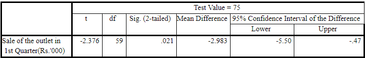
One Sample Test Table shows the result of the t-test. Here, test statistic value (from the sample) is t = -2.376 and the corresponding p-value (2 tailed) = 0.021 <0.05. So, H 0 got rejected and it can be said that the claim of average first quarterly sales being 75 (thousand) does not hold. 

Two Independent Samples t-Test

• Analyze => Compare Means => Independent-Samples T-Test to open the dialogue box.
• Enter the Test variable (variable under consideration) in the Test Variable(s) box and variable categorising the groups in the Grouping Variable box.
• Define the groups by clicking on Define Groups and enter the relevant numeric-codes into the relevant groups in the Define Groups sub-dialogue box. Press Continue to return back to the main dialogue box.

We continue with the example of Ventura Sales, and want to compare the average first quarter sales with respect to Urban Outlets and Rural Outlets (two independent samples/groups). Here, the claim is that urban outlets are giving lower sales as compared to rural outlets. So, the Hypotheses:

H 0 : µ 1 – µ 2 = 0 or µ 1 = µ 2   (Where, µ 1 = Population Mean Sale of Urban Outlets and µ 2 = Population Mean Sale of Rural Outlets)

H 1 : µ 1 < µ 2  

Group Statistics

Descriptive table showing the sample sizes n 1 =37 and n 2 =23, sample means x̄ 1 =67.86 and x̄ 2 =78.70, sample standard deviations s 1 =8.570 and s 2 = 7.600.

The below table is the Independent Sample Test Table, proving all the relevant test statistics and p-values.  Here, both the outputs for Equal Variance (assumed) and Unequal Variance (assumed) are presented.

Independent Samples Test

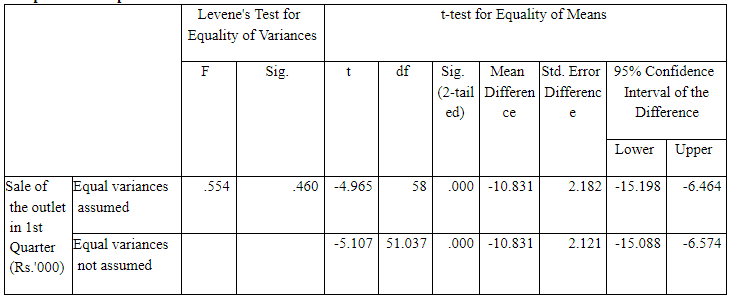
So, we have to figure out whether we should go for ‘equal variance’ case or for ‘unequal variances’ case. 

Here, Levene’s Test for Equality of Variances has to be applied for this purpose with the hypotheses: H 0 : σ² 1 = σ² 2 and H 1 : σ² 1 ≠ σ² 2 . The p-value (Sig) = 0.460 >0.05, so we can’t reject (so retained) H 0 . Hence, variances can be assumed to be equal. 

So, “Equal Variances assumed” case is to be taken up. Accordingly, the value of t statistic = -4.965 and the p-value (two tailed) = 0.000, so the p-value (one tailed) = 0.000/2 = 0.000 <0.05. Hence, H 0 got rejected and it can be said that urban outlets are giving lower sales in the first quarter. So, the claim stands.

Paired t-Test (Testing Difference between Means with Dependent Samples):

•   Analyze => Compare Means => Paired-Samples T-Test to open the dialogue box.
• Enter the relevant pair of variables (paired samples) in the Paired Variables box.
• After entering the paired samples, press Ok to have the output.

We continue with the example of Ventura Sales, and want to compare the average first quarter sales with the second quarter sales. Some sales promotion interventions were executed with an expectation of increasing sales in the second quarter. So, the Hypotheses:

H 0 : µ 1 = µ 2 (Where, µ 1 = Population Mean Sale of Quarter-I and µ 2 = Population Mean Sale of Quarter-II)

H 1 : µ 1 < µ 2 (representing the increase of sales i.e. implying the success of sales interventions)

Paired Samples Statistics

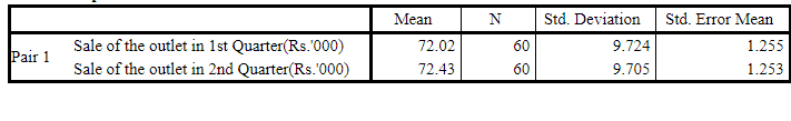
Descriptive table showing the sample size n=60, sample means x̄ 1 =72.02 and x̄ 2 =72.43.

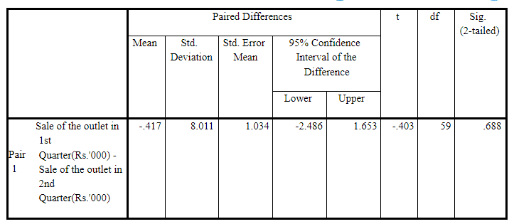
As per the following output table (Paired Samples Test), sample mean of differences d̅ = -0.417 with standard deviation of differences sd = 8.011 and value of t statistic = -0.403. Accordingly, the p-value (two tailed) = 0.688, so the p-value (one tailed) = 0.688/2 = 0.344 > 0.05. So, there have not been sufficient reasons to Reject H 0 i.e. H 0 should be retained. So, the effectiveness (success) of the sales promotion interventions is doubtful i.e. it didn’t result in significant increase in sales, provided all other extraneous factors remain the same.

Paired Samples Test   

t-Test Application One Sample

Experience Marketing Services reported that the typical American spends a mean of 144 minutes (2.4 hours) per day accessing the Internet via a mobile device. (Source: The 2014 Digital Marketer, available at ex.pn/1kXJifX.) To test the validity of this statement, you select a sample of 30 friends and family. The result for the time spent per day accessing the Internet via a mobile device (in minutes) are stored in Internet_Mobile_Time.csv file.

Is there evidence that the populations mean time spent per day accessing the Internet via a mobile device is different from 144 minutes? Use the p-value approach and a level of significance of 0.05

What assumption about the population distribution is needed to conduct the test in A?

Solution In R

[1] 1.224674

[1] 0.2305533

[1] “Accepted”

Independent t-test two sample

A hotel manager looks to enhance the initial impressions that hotel guests have when they check-in. Contributing to initial impressions is the time it takes to deliver a guest’s luggage to the room after check-in. A random sample of 20 deliveries on a particular day was selected each from Wing A and Wing B of the hotel. The data collated is given in Luggage.csv file. Analyze the data and determine whether there is a difference in the mean delivery times in the two wings of the hotel. (use alpha = 0.05).

    Two Sample t-test data:  WingA and WingB t = 5.1615, df = 38, p-value = 4.004e-06 alternative hypothesis: true difference in means is greater than 0 95 percent confidence interval: 1.531895   Inf sample estimates: mean of x mean of y  10.3975 8.1225 > t.test(WingA,WingB)    Welch Two Sample t-test

t = 5.1615, df = 37.957, p-value = 8.031e-06 alternative hypothesis: true difference in means is not equal to 0 95 per cent confidence interval: 1.38269 3.16731 sample estimates: mean of x mean of y  10.3975 8.1225

Case Study- Titan Insurance Company

The Titan Insurance Company has just installed a new incentive payment scheme for its lift policy salesforce. It wants to have an early view of the success or failure of the new scheme. Indications are that the sales force is selling more policies, but sales always vary in an unpredictable pattern from month to month and it is not clear that the scheme has made a significant difference.

Life Insurance companies typically measure the monthly output of a salesperson as the total sum assured for the policies sold by that person during the month. For example, suppose salesperson X has, in the month, sold seven policies for which the sums assured are £1000, £2500, £3000, £5000, £10000, £35000. X’s output for the month is the total of these sums assured, £61,500.

Titan’s new scheme is that the sales force receives low regular salaries but are paid large bonuses related to their output (i.e. to the total sum assured of policies sold by them). The scheme is expensive for the company, but they are looking for sales increases which more than compensate. The agreement with the sales force is that if the scheme does not at least break even for the company, it will be abandoned after six months.

The scheme has now been in operation for four months. It has settled down after fluctuations in the first two months due to the changeover.

To test the effectiveness of the scheme, Titan has taken a random sample of 30 salespeople measured their output in the penultimate month before changeover and then measured it in the fourth month after the changeover (they have deliberately chosen months not too close to the changeover). Ta ble 1 shows t he outputs of the salespeople in Table 1

Data preparation

Since the given data are in 000, it will be better to convert them in thousands. Problem 1 Describe the five per cent significance test you would apply to these data to determine whether the new scheme has significantly raised outputs? What conclusion does the test lead to? Solution: It is asked that whether the new scheme has significantly raised the output, it is an example of the one-tailed t-test. Note: Two-tailed test could have been used if it was asked “new scheme has significantly changed the output” Mean of amount assured before the introduction of scheme = 68450 Mean of amount assured after the introduction of scheme = 72000 Difference in mean = 72000 – 68450 = 3550 Let, μ1 = Average sums assured by salesperson BEFORE changeover. μ2 = Average sums assured by salesperson AFTER changeover. H0: μ1 = μ2  ; μ2 – μ1 = 0 HA: μ1 < μ2   ; μ2 – μ1 > 0 ; true difference of means is greater than zero. Since population standard deviation is unknown, paired sample t-test will be used.

Since p-value (=0.06529) is higher than 0.05, we accept (fail to reject) NULL hypothesis. The new scheme has NOT significantly raised outputs .

Problem 2 Suppose it has been calculated that for Titan to break even, the average output must increase by £5000. If this figure is an alternative hypothesis, what is: (a)  The probability of a type 1 error? (b)  What is the p-value of the hypothesis test if we test for a difference of $5000? (c)   Power of the test: Solution: 2.a.  The probability of a type 1 error? Solution: Probability of Type I error = significant level = 0.05 or 5% 2.b.  What is the p-value of the hypothesis test if we test for a difference of $5000? Solution: Let  μ2 = Average sums assured by salesperson AFTER changeover. μ1 = Average sums assured by salesperson BEFORE changeover. μd = μ2 – μ1   H0: μd ≤ 5000 HA: μd > 5000 This is a right tail test.

P-value = 0.6499 2.c. Power of the test. Solution: Let  μ2 = Average sums assured by salesperson AFTER changeover. μ1 = Average sums assured by salesperson BEFORE changeover. μd = μ2 – μ1   H0: μd = 4000 HA: μd > 0

H0 will be rejected if test statistics > t_critical. With α = 0.05 and df = 29, critical value for t statistic (or t_critical ) will be   1.699127. Hence, H0 will be rejected for test statistics ≥  1.699127. Hence, H0 will be rejected if for  𝑥̅ ≥ 4368.176

Graphically,

      Probability (type II error) is P(Do not reject H0 | H0 is false)       Our NULL hypothesis is TRUE at μd = 0 so that  H0: μd = 0 ; HA: μd > 0       Probability of type II error at μd = 5000

= P (Do not reject H0 | H0 is false) = P (Do not reject H0 | μd = 5000)  = P (𝑥̅ < 4368.176 | μd = 5000) = P (t <  | μd = 5000) = P (t < -0.245766) = 0.4037973

R Code: Now,  β=0.5934752, Power of test = 1- β = 1- 0.5934752 = 0.4065248

• While performing Hypothesis-Testing, Hypotheses can’t be proved or disproved since we have evidence from sample (s) only. At most, Hypotheses may be rejected or retained.
• Use of the term “accept H 0 ” in place of “do not reject” should be avoided even if the test statistic falls in the Acceptance Region or p-value ≥ α. This simply means that the sample does not provide sufficient statistical evidence to reject the H 0 . Since we have tried to nullify (reject) H 0 but we haven’t found sufficient support to do so, we may retain it but it won’t be accepted.
• Confidence Interval (Interval Estimation) can also be used for testing of hypotheses. If the hypothesis parameter falls within the confidence interval, we do not reject H 0 . Otherwise, if the hypothesised parameter falls outside the confidence interval i.e. confidence interval does not contain the hypothesized parameter, we reject H 0 .
• Downey, A. B. (2014). Think Stat: Exploratory Data Analysis , 2 nd Edition, Sebastopol, CA: O’Reilly Media Inc
• Fisher, R. A. (1956). Statistical Methods and Scientific Inference , New York: Hafner Publishing Company.
• Hogg, R. V.; McKean, J. W. & Craig, A. T. (2013). Introduction to Mathematical Statistics , 7 th Edition, New Delhi: Pearson India.
• IBM SPSS Statistics. (2020). IBM Corporation. 
• Levin, R. I.; Rubin, D. S; Siddiqui, M. H. & Rastogi, S. (2017). Statistics for Management , 8 th Edition, New Delhi: Pearson India. 

If you want to get a detailed understanding of Hypothesis testing, you can take up this hypothesis testing in machine learning course. This course will also provide you with a certificate at the end of the course.

If you want to learn more about R programming and other concepts of Business Analytics or Data Science, sign up for Great Learning ’s PG program in Data Science and Business Analytics.

Top Free Courses

Top 30 Python Libraries To Know

Python Dictionary Append: How To Add Key/Value Pair?

¿Qué es la Ciencia de Datos? – Una Guía Completa [2024]

What is Data Science? – The Complete Guide

What is Time Complexity And Why Is It Essential?

Python NumPy Tutorial – 2024

Leave a comment cancel reply.

Your email address will not be published. Required fields are marked *

Save my name, email, and website in this browser for the next time I comment.

Table of contents

• Business Essentials
• Leadership & Management
• Credential of Leadership, Impact, and Management in Business (CLIMB)
• Entrepreneurship & Innovation
• Digital Transformation
• Finance & Accounting
• Business in Society
• For Organizations
• Support Portal
• Media Coverage
• Founding Donors
• Leadership Team

• Harvard Business School →
• HBS Online →
• Business Insights →

Business Insights

Harvard Business School Online's Business Insights Blog provides the career insights you need to achieve your goals and gain confidence in your business skills.

• Career Development
• Communication
• Decision-Making
• Earning Your MBA
• Negotiation
• News & Events
• Productivity
• Staff Spotlight
• Student Profiles
• Work-Life Balance
• AI Essentials for Business
• Alternative Investments
• Business Analytics
• Business Strategy
• Business and Climate Change
• Design Thinking and Innovation
• Digital Marketing Strategy
• Disruptive Strategy
• Economics for Managers
• Entrepreneurship Essentials
• Financial Accounting
• Global Business
• Launching Tech Ventures
• Leadership Principles
• Leadership, Ethics, and Corporate Accountability
• Leading with Finance
• Management Essentials
• Negotiation Mastery
• Organizational Leadership
• Power and Influence for Positive Impact
• Strategy Execution
• Sustainable Business Strategy
• Sustainable Investing
• Winning with Digital Platforms

A Beginner’s Guide to Hypothesis Testing in Business

• 30 Mar 2021

Becoming a more data-driven decision-maker can bring several benefits to your organization, enabling you to identify new opportunities to pursue and threats to abate. Rather than allowing subjective thinking to guide your business strategy, backing your decisions with data can empower your company to become more innovative and, ultimately, profitable.

If you’re new to data-driven decision-making, you might be wondering how data translates into business strategy. The answer lies in generating a hypothesis and verifying or rejecting it based on what various forms of data tell you.

Below is a look at hypothesis testing and the role it plays in helping businesses become more data-driven.

Access your free e-book today.

What Is Hypothesis Testing?

To understand what hypothesis testing is, it’s important first to understand what a hypothesis is.

A hypothesis or hypothesis statement seeks to explain why something has happened, or what might happen, under certain conditions. It can also be used to understand how different variables relate to each other. Hypotheses are often written as if-then statements; for example, “If this happens, then this will happen.”

Hypothesis testing , then, is a statistical means of testing an assumption stated in a hypothesis. While the specific methodology leveraged depends on the nature of the hypothesis and data available, hypothesis testing typically uses sample data to extrapolate insights about a larger population.

Hypothesis Testing in Business

When it comes to data-driven decision-making, there’s a certain amount of risk that can mislead a professional. This could be due to flawed thinking or observations, incomplete or inaccurate data , or the presence of unknown variables. The danger in this is that, if major strategic decisions are made based on flawed insights, it can lead to wasted resources, missed opportunities, and catastrophic outcomes.

The real value of hypothesis testing in business is that it allows professionals to test their theories and assumptions before putting them into action. This essentially allows an organization to verify its analysis is correct before committing resources to implement a broader strategy.

As one example, consider a company that wishes to launch a new marketing campaign to revitalize sales during a slow period. Doing so could be an incredibly expensive endeavor, depending on the campaign’s size and complexity. The company, therefore, may wish to test the campaign on a smaller scale to understand how it will perform.

In this example, the hypothesis that’s being tested would fall along the lines of: “If the company launches a new marketing campaign, then it will translate into an increase in sales.” It may even be possible to quantify how much of a lift in sales the company expects to see from the effort. Pending the results of the pilot campaign, the business would then know whether it makes sense to roll it out more broadly.

Related: 9 Fundamental Data Science Skills for Business Professionals

Key Considerations for Hypothesis Testing

1. alternative hypothesis and null hypothesis.

In hypothesis testing, the hypothesis that’s being tested is known as the alternative hypothesis . Often, it’s expressed as a correlation or statistical relationship between variables. The null hypothesis , on the other hand, is a statement that’s meant to show there’s no statistical relationship between the variables being tested. It’s typically the exact opposite of whatever is stated in the alternative hypothesis.

For example, consider a company’s leadership team that historically and reliably sees $12 million in monthly revenue. They want to understand if reducing the price of their services will attract more customers and, in turn, increase revenue.

In this case, the alternative hypothesis may take the form of a statement such as: “If we reduce the price of our flagship service by five percent, then we’ll see an increase in sales and realize revenues greater than $12 million in the next month.”

The null hypothesis, on the other hand, would indicate that revenues wouldn’t increase from the base of $12 million, or might even decrease.

Check out the video below about the difference between an alternative and a null hypothesis, and subscribe to our YouTube channel for more explainer content.

2. Significance Level and P-Value

Statistically speaking, if you were to run the same scenario 100 times, you’d likely receive somewhat different results each time. If you were to plot these results in a distribution plot, you’d see the most likely outcome is at the tallest point in the graph, with less likely outcomes falling to the right and left of that point.

With this in mind, imagine you’ve completed your hypothesis test and have your results, which indicate there may be a correlation between the variables you were testing. To understand your results' significance, you’ll need to identify a p-value for the test, which helps note how confident you are in the test results.

In statistics, the p-value depicts the probability that, assuming the null hypothesis is correct, you might still observe results that are at least as extreme as the results of your hypothesis test. The smaller the p-value, the more likely the alternative hypothesis is correct, and the greater the significance of your results.

3. One-Sided vs. Two-Sided Testing

When it’s time to test your hypothesis, it’s important to leverage the correct testing method. The two most common hypothesis testing methods are one-sided and two-sided tests , or one-tailed and two-tailed tests, respectively.

Typically, you’d leverage a one-sided test when you have a strong conviction about the direction of change you expect to see due to your hypothesis test. You’d leverage a two-sided test when you’re less confident in the direction of change.

4. Sampling

To perform hypothesis testing in the first place, you need to collect a sample of data to be analyzed. Depending on the question you’re seeking to answer or investigate, you might collect samples through surveys, observational studies, or experiments.

A survey involves asking a series of questions to a random population sample and recording self-reported responses.

Observational studies involve a researcher observing a sample population and collecting data as it occurs naturally, without intervention.

Finally, an experiment involves dividing a sample into multiple groups, one of which acts as the control group. For each non-control group, the variable being studied is manipulated to determine how the data collected differs from that of the control group.

Learn How to Perform Hypothesis Testing

Hypothesis testing is a complex process involving different moving pieces that can allow an organization to effectively leverage its data and inform strategic decisions.

If you’re interested in better understanding hypothesis testing and the role it can play within your organization, one option is to complete a course that focuses on the process. Doing so can lay the statistical and analytical foundation you need to succeed.

Do you want to learn more about hypothesis testing? Explore Business Analytics —one of our online business essentials courses —and download our Beginner’s Guide to Data & Analytics .

About the Author

An official website of the United States government

The .gov means it’s official. Federal government websites often end in .gov or .mil. Before sharing sensitive information, make sure you’re on a federal government site.

The site is secure. The https:// ensures that you are connecting to the official website and that any information you provide is encrypted and transmitted securely.

• Publications
• Account settings

Preview improvements coming to the PMC website in October 2024. Learn More or Try it out now .

• Advanced Search
• Journal List
• Ind Psychiatry J
• v.18(1); Jan-Jun 2009

Probability, clinical decision making and hypothesis testing

A. banerjee.

Department of Community Medicine, D. Y. Patil Medical College, Pune - 411018, India

S. L. Jadhav

J. s. bhawalkar.

Few clinicians grasp the true concept of probability expressed in the ‘ P value.’ For most, a statistically significant P value is the end of the search for truth. In fact, the opposite is the case. The present paper attempts to put the P value in proper perspective by explaining different types of probabilities, their role in clinical decision making, medical research and hypothesis testing.

The clinician who wishes to remain abreast with the results of medical research needs to develop a statistical sense. He reads a number of journal articles; and constantly, he must ask questions such as, “Am I convinced that lack of mental activity predisposes to Alzheimer’s? Or “Do I believe that a particular drug cures more patients than the drug I use currently?”

The results of most studies are quantitative; and in earlier times, the reader made up his mind whether or not to accept the results of a particular study by merely looking at the figures. For instance, if 25 out of 30 patients were cured with a new drug compared with 15 out of the 30 on placebo, the superiority of the new drug was readily accepted.

In recent years, the presentation of medical research has undergone much transformation. Nowadays, no respectable journal will accept a paper if the results have not been subjected to statistical significance tests. The use of statistics has accelerated with the ready availability of statistical software. It has now become fashionable to organize workshops on research methodology and biostatistics. No doubt, this development was long overdue and one concedes that the methodologies of most medical papers have considerably improved in recent years. But at the same time, a new problem has arisen. The reading of medical journals today presupposes considerable statistical knowledge; however, those doctors who are not familiar with statistical theory tend to interpret the results of significance tests uncritically or even incorrectly.

It is often overlooked that the results of a statistical test depend not only on the observed data but also on the choice of statistical model. The statistician doing analysis of the data has a choice between several tests which are based on different models and assumptions. Unfortunately, many research workers who know little about statistics leave the statistical analysis to statisticians who know little about medicine; and the end result may well be a series of meaningless calculations.

Many readers of medical journals do not know the correct interpretation of ‘ P values,’ which are the results of significance tests. Usually, it is only stated whether the P value is below 5% ( P < .05) or above 5% ( P > .05). According to convention, the results of P < .05 are said to be statistically significant, and those with P > .05 are said to be statistically nonsignificant. These expressions are taken so seriously by most that it is almost considered ‘unscientific’ to believe in a nonsignificant result or not to believe in a ‘significant’ result. It is taken for granted that a ‘significant’ difference is a true difference and that a ‘nonsignificant’ difference is a chance finding and does not merit further exploration. Nothing can be further from the truth.

The present paper endeavors to explain the meaning of probability, its role in everyday clinical practice and the concepts behind hypothesis testing.

WHAT IS PROBABILITY?

Probability is a recurring theme in medical practice. No doctor who returns home from a busy day at the hospital is spared the nagging feeling that some of his diagnoses may turn out to be wrong, or some of his treatments may not lead to the expected cure. Encountering the unexpected is an occupational hazard in clinical practice. Doctors after some experience in their profession reconcile to the fact that diagnosis and prognosis always have varying degrees of uncertainty and at best can be stated as probable in a particular case.

Critical appraisal of medical journals also leads to the same gut feeling. One is bombarded with new research results, but experience dictates that well-established facts of today may be refuted in some other scientific publication in the following weeks or months. When a practicing clinician reads that some new treatment is superior to the conventional one, he will assess the evidence critically, and at best he will conclude that probably it is true.

Two types of probabilities

The statistical probability concept is so widely prevalent that almost everyone believes that probability is a frequency . It is not, of course, an ordinary frequency which can be estimated by simple observations, but it is the ideal or truth in the universe , which is reflected by the observed frequency. For example, when we want to determine the probability of obtaining an ace from a pack of cards (which, let us assume has been tampered with by a dishonest gambler), we proceed by drawing a card from the pack a large number of times, as we know in the long run, the observed frequency will approach the true probability or truth in the universe. Mathematicians often state that a probability is a long-run frequency, and a probability that is defined in this way is called a frequential probability . The exact magnitude of a frequential probability will remain elusive as we cannot make an infinite number of observations; but when we have made a decent number of observations (adequate sample size), we can calculate the confidence intervals, which are likely to include the true frequential probability. The width of the confidence interval depends on the number of observations (sample size).

The frequential probability concept is so prevalent that we tend to overlook terms like chance, risk and odds, in which the term probability implies a different meaning. Few hypothetical examples will make this clear. Consider the statement, “The cure for Alzheimer’s disease will probably be discovered in the coming decade.” This statement does not indicate the basis of this expectation or belief as in frequential probability, where a number of repeated observations provide the foundation for probability calculation. However, it may be based on the present state of research in Alzheimer’s. A probabilistic statement incorporates some amount of uncertainty, which may be quantified as follows: A politician may state that there is a fifty-fifty chance of winning the next election, a bookie may say that the odds of India winning the next one-day cricket game is four to one, and so on. At first glance, such probabilities may appear frequential ones, but a little reflection will reveal the contrary. We are concerned with unique events, i.e., the likely cure of a disease in the future, the next particular election, the next particular one-day game — and it makes no sense to apply the statistical idea that these types of probabilities are long-run frequencies. Further reflection will illustrate that these statements about probabilities of the election and one-day game are no different from the one about the cure for Alzheimer’s, apart from the fact that in the latter cases an attempt has been made to quantify the magnitude of belief in the occurrence of the event.

It follows from the above deliberations that we have 2 types of probability concepts. In the jargon of statistics, a probability is ideal or truth in the universe which lies beneath an observed frequency — such probabilities may be called frequential probabilities. In literary language, a probability is a measure of our subjective belief in the occurrence of a particular event or truth of a hypothesis. Such probabilities, which may be quantified that they look like frequential ones, are called subjective probabilities. Bayesian statistical theory also takes into account subjective probabilities (Lindley, 1973; Winkler, 1972). The following examples will try to illustrate these (rather confusing) concepts.

A young man is brought to the psychiatry OPD with history of withdrawal. He also gives history of talking to himself and giggling without cause. There is also a positive family history of schizophrenia. The consulting psychiatrist who examines the patient concludes that there is a 90% probability that this patient suffers from schizophrenia.

We ask the psychiatrist what makes him make such a statement. He may not be able to say that he knows from experience that 90% of such patients suffer from schizophrenia. The statement therefore may not be based on observed frequency. Instead, the psychiatrist states his probability based on his knowledge of the natural history of disease and the available literature regarding signs and symptoms in schizophrenia and positive family history. From this knowledge, the psychiatrist concludes that his belief in the diagnosis of schizophrenia in that particular patient is as strong as his belief in picking a black ball from a box containing 10 white and 90 black balls. The probability in this case is certainly subjective probability .

Let us consider another example: A 26-year-old married female patient who suffered from severe abdominal pain is referred to a hospital. She is also having amenorrhea for the past 4 months. The pain is located in the left lower abdomen. The gynecologist who examines her concludes that there is a 30% probability that the patient is suffering from ectopic pregnancy.

As before, we ask the gynecologist to explain on what basis the diagnosis of ectopic pregnancy is suspected. In this case the gynecologist states that he has studied a large number of successive patients with this symptom complex of lower abdominal pain with amenorrhea, and that a subsequent laparotomy revealed an ectopic pregnancy in 30% of the cases.

If we accept that the study cited is large enough to make us assume that the possibility of the observed frequency of ectopic pregnancy did not differ from the true frequential probability, it is natural to conclude that the gynecologist’s probability claim is more ‘evidence based’ than that of the psychiatrist, but again this is debatable.

In order to grasp this in proper perspective, it is necessary to note that the gynecologist stated that the probability of ectopic pregnancy in that particular patient was 30%. Therefore, we are concerned with a unique event just as the politician’s next election or India’s next one-day match. So in this case also, the probability is a subjective probability which was based on an observed frequency . One might also argue that even this probability is not good enough. We might ask the gynecologist to base his belief on a group of patients who also had the same age, height, color of hair and social background; and in the end, the reference group would be so restrictive that even the experience from a very large study would not provide the necessary information. If we went even further and required that he must base his belief on patients who in all respects resembled this particular patient, the probabilistic problem would vanish as we will be dealing with a certainty rather than a probability.

The clinician’s belief in a particular diagnosis in an individual patient may be based on the recorded experience in a group of patients, but it is still a subjective probability. It reflects not only the observed frequency of the disease in a reference group but also the clinician’s theoretical knowledge which determines the choice of reference group (Wulff, Pedersen and Rosenberg, 1986). Recorded experience is never the sole basis of clinical decision making.

GAP BETWEEN THEORY AND PRACTICE

The two situations described above are relatively straightforward. The physician observed a patient with a particular set of signs and symptoms and assessed the subjective probability about the diagnosis in each case. Such probabilities have been termed diagnostic probabilities (Wulff, Pedersen and Rosenberg, 1986). In practice, however, clinicians make diagnosis in a more complex manner which they themselves may be unable to analyze logically.

For instance, suppose the clinician suspects one of his patients is suffering from a rare disease named ‘D.’ He requests a suitable test to confirm the diagnosis, and suppose the test is positive for disease ‘D.’ He now wishes to assess the probability of the diagnosis being positive on the basis of this information, but perhaps the medical literature only provides the information that a positive test is seen in 70% of the patients with disease ‘D.’ However, it is also positive in 2% of patients without disease ‘D.’ How to tackle this doctor’s dilemma? First a formal analysis may be attempted, and then we can return to everyday clinical thinking. The frequential probability which the doctor found in the literature may be written in the statistical notation as follows:

P (S/D+) = .70, i.e., the probability of the presence of this particular sign (or test) given this particular disease is 70%.

P (S/D–) = .02, i.e., the probability of this particular sign given the absence of this particular disease is 2%.

However, such probabilities are of little clinical relevance. The clinical relevance is in the ‘opposite’ probability. In clinical practice, one would like to know the P (D/S), i.e., the probability of the disease in a particular patient given this positive sign. This can be estimated by means of Bayes’ Theorem (Papoulis, 1984; Lindley, 1973; Winkler, 1972). The formula of Bayes’ Theorem is reproduced below, from which it will be evident that to calculate P(D/S), we must also know the prior probability of the presence and the absence of the disease, i.e., P (D+) and P (D–).

P (D/S) = P (S/D+) P (D+) ÷ P (S/D+) P (D+) + P (S/D–) P (D–)

In the example of the disease ‘D’ above, let us assume that we estimate that prior probability of the disease being present, i.e., P (D+), is 25%; and therefore, prior probability of the absence of disease, i.e., P (D–), is 75%. Using the Bayes’ Theorem formula, we can calculate that the probability of the disease given a positive sign, i.e., P (D/S), is 92%.

We of course do not suggest that clinicians should always make calculations of this sort when confronted with a diagnostic dilemma, but they must in an intuitive way think along these lines. Clinical knowledge is to a large extent based on textbook knowledge, and ordinary textbooks do not tell the reader much about the probabilities of different diseases given different symptoms. Bayes’ Theorem guides a clinician how to use textbook knowledge for practical clinical purposes.

The practical significance of this point is illustrated by the European doctor who accepted a position at a hospital in tropical Africa. In order to prepare himself for the new job, he bought himself a large textbook of tropical medicine and studied in great detail the clinical pictures of a large number of exotic diseases. However, for several months after his arrival at the tropical hospital, his diagnostic performance was very poor, as he knew nothing about the relative frequency of all these diseases. He had to acquaint himself with the prior probability, P (D +), of the diseases in the catchment area of the hospital before he could make precise diagnoses.

The same thing happens on a smaller scale when a doctor trained at a university hospital establishes himself in general practice. At the beginning, he will suspect his patients of all sorts of rare diseases (which are common at the university hospital), but after a while he will learn to assess correctly the frequency of different diseases in the general population.

PROBABILITY AND HYPOTHESIS TESTING

Besides predictions on individual patients, the doctor is also concerned in generalizations to the population at large or the target population. We may say that probably there may have been life at Mars. We may even quantify our belief and mention that there is 95% probability that depression responds more quickly during treatment with a particular antidepressant than during treatment with a placebo. These probabilities are again subjective probabilities rather than frequential probabilities . The last statement does not imply that 95% of depression cases respond to the particular antidepressant or that 95% of the published reports mention that the particular antidepressant is the best. It simply means that our belief in the truth of the statement is the same as our belief in picking up a red ball from a box containing 95 red balls and 5 white balls. It means that we are, however, almost not totally convinced that the average recovery time during treatment with a particular antidepressant is shorter than during placebo treatment.

The purpose of hypothesis testing is to aid the clinician in reaching a conclusion concerning the universe by examining a sample from that universe. A hypothesis may be defined as a presumption or statement about the truth in the universe. For example, a clinician may hypothesize that a certain drug may be effective in 80% of the cases of schizophrenia. It is frequently concerned about the parameters in the population about which the presumption or statement is made. It is the basis for motivating the research project. There are two types of hypotheses, research hypothesis and statistical hypothesis (Daniel, 2000; Guyatt et al ., 1995).

Genesis of research hypothesis

Hypothesis may be generated by deduction from anatomical, physiological facts or from clinical observations.

Statistical hypothesis

Statistical hypotheses are hypotheses that are stated in such a way that they may be evaluated by appropriate statistical techniques.

Pre-requisites for hypothesis testing

Nature of data.

The types of data that form the basis of hypothesis testing procedures must be understood, since these dictate the choice of statistical test.

Presumptions

These presumptions are the normality of the population distribution, equality of the standard deviations, random samples.

There are 2 statistical hypotheses involved in hypothesis testing. These should be stated a priori and explicitly. The null hypothesis is the hypothesis to be tested. It is denoted by the symbol H 0 . It is also known as the hypothesis of no difference . The null hypothesis is set up with the sole purpose of efforts to knock it down. In the testing of hypothesis, the null hypothesis is either rejected (knocked down) or not rejected (upheld). If the null hypothesis is not rejected, the interpretation is that the data is not sufficient evidence to cause rejection. If the testing process rejects the null hypothesis, the inference is that the data available to us is not compatible with the null hypothesis and by default we accept the alternative hypothesis , which in most cases is the research hypothesis. The alternative hypothesis is designated with the symbol H A .

Limitations

Neither hypothesis testing nor statistical tests lead to proof. It merely indicates whether the hypothesis is supported or not supported by the available data. When we reject a null hypothesis, we do not mean it is not true but that it may be true. By default when we do not reject the null hypothesis, we should have this limitation in mind and should not convey the impression that this implies proof.

Test statistic

The test statistic is the statistic that is derived from the data from the sample. Evidently, many possible values of the test statistic can be computed depending on the particular sample selected. The test statistic serves as a decision maker, nothing more, nothing less, rather than proof or lack of it. The decision to reject or not to reject the null hypothesis depends on the magnitude of the test statistic.

Types of decision errors

The error committed when a true null hypothesis is rejected is called the type I error or α error . When a false null hypothesis is not rejected, we commit type II error, or β error . When we reject a null hypothesis, there is always the risk (howsoever small it may be) of committing a type I error, i.e., rejecting a true null hypothesis. On the other hand, whenever we fail to reject a null hypothesis, the risk of failing to reject a false null hypothesis, or committing a type II error, will always be present. Put in other words, the test statistic does not eliminate uncertainty (as many tend to believe); it only quantifies our uncertainty.

Calculation of test statistic

From the data contained in the sample, we compute a value of the test statistic and compare it with the rejection and non-rejection regions, which have to be specified in advance.

Statistical decision

The statistical decision consists of rejecting or of not rejecting the null hypothesis. It is rejected if the computed value of the test statistic falls in the rejection region, and it is not rejected if the value falls in the non-rejection region.

If H 0 is rejected, we conclude that H A is true. If H 0 is not rejected, we conclude that H 0 may be true.

The P value is a number that tells us how unlikely our sample values are, given that the null hypothesis is true. A P value indicating that the sample results are not likely to have occurred, if the null hypothesis is true, provides reason for doubting the truth of the null hypothesis.

We must remember that, when the null hypothesis is not rejected, one should not say the null hypothesis is accepted. We should mention that the null hypothesis is “not rejected.” We avoid using the word accepted in this case because we may have committed a type II error. Since, frequently, the probability of committing error can be quite high (particularly with small sample sizes), we should not commit ourselves to accepting the null hypothesis.

INTERPRETATIONS

With the above discussion on probability, clinical decision making and hypothesis testing in mind, let us reconsider the meaning of P values. When we come across the statement that there is statistically significant difference between two treatment regimes with P < .05, we should not interpret that there is less than 5% probability that there is no difference, and that there is 95% probability that a difference exists, as many uninformed readers tend to do. The statement that there is difference between the cure rates of two treatments is a general one, and we have already discussed that the probability of the truth of a general statement (hypothesis) is subjective , whereas the probabilities which are calculated by statisticians are frequential ones. The hypothesis that one treatment is better than the other is either true or false and cannot be interpreted in frequential terms.

To explain this further, suppose someone claims that 20 (80%) of 25 patients who received drug A were cured, compared to 12 (48%) of 25 patients who received drug B. In this case, there are two possibilities, either the null hypothesis is true, which means that the two treatments are equally effective and the observed difference arose by chance; or the null hypothesis is not true (and we accept the alternative hypothesis by default), which means that one treatment is better than the other. The clinician wants to make up his mind to what extent he believes in the truth of the alternative hypothesis (or the falsehood of the null hypothesis ). To resolve this issue, he needs the aid of statistical analysis. However, it is essential to note that the P value does not provide a direct answer. Let us assume in this case the statistician does a significance test and gets a P value = .04, meaning that the difference is statistically significant ( P < .05). But as explained earlier, this does not mean that there is a 4% probability that the null hypothesis is true and 96% chance that the alternative hypothesis is true. The P value is a frequential probability and it provides the information that there is a 4% probability of obtaining such a difference between the cure rates, if the null hypothesis is true . In other words, the statistician asks us to assume that the null hypothesis is true and to imagine that we do a large number of trials. In that case, the long-run frequency of trials which show a difference between the cure rates like the one we found, or even a larger one, will be 4%.

Prior belief and interpretation of the P value

In order to elucidate the implications of the correct statistical definition of the P value, let us imagine that the patients who took part in the above trial suffered from depression, and that drug A was gentamycin, while drug B was a placebo. Our theoretical knowledge gives us no grounds for believing that gentamycin has any affect whatsoever in the cure of depression. For this reason, our prior confidence in the truth of the null hypothesis is immense (say, 99.99%), whereas our prior confidence in the alternative hypothesis is minute (0.01%). We must take these prior probabilities into account when we assess the result of the trial. We have the following choice. Either we accept the null hypothesis in spite of the fact that the probability of the trial result is fairly low at 4% ( P < .05) given the null hypothesis is true, or we accept the alternative hypothesis by rejecting the null hypothesis in spite of the fact that the subjective probability of that hypothesis is extremely low in the light of our prior knowledge.

It will be evident that the choice is a difficult one, as both hypotheses, each in its own way, may be said to be unlikely, but any clinician who reasons along these lines will choose that hypothesis which is least unacceptable: He will accept the null hypothesis and claim that the difference between the cure rates arose by chance (however small it may be), as he does not feel that the evidence from this single trial is sufficient to shake his prior belief in the null hypothesis.

Misinterpretation of P values is extremely common. One of the reasons may be that those who teach research methods do not themselves appreciate the problem. The P value is the probability of obtaining a value of the test statistic as large as or larger than the one computed from the data when in reality there is no difference between the different treatments. In other words, the P value is the probability of being wrong when asserting that a difference exists.

Lastly, we must remember we do not establish proof by hypothesis testing, and uncertainty will always remain in empirical research; at the most, we can only quantify our uncertainty.

Source of Support: Nil

Conflict of Interest: None declared.

Navigation Menu

Search code, repositories, users, issues, pull requests..., provide feedback.

We read every piece of feedback, and take your input very seriously.

Saved searches

Use saved searches to filter your results more quickly.

To see all available qualifiers, see our documentation .

• Notifications

AayushKulshrestha/Hypothesis-Testing-Case-Study

Folders and files, repository files navigation, hypothesis-testing-case-study.

BUSINESS PROBLEM: Using lending club loans data, the team would like to test below hypothesis on how different factors effecing each other (Hint: You may leverage hypothesis testing using statistical tests)

BUSINESS PROBLEM: We would like to assess if there is any difference in the average price quotes provided by Mary and Barry.

BUSINESS PROBLEM: Determine what effect, if any, the reengineering effort had on the incidence behavioral problems and staff turnover. i.e To determine if the reengineering effortchanged the critical incidence rate. Is there evidence that the critical incidence rate improved?

BUSINESS PROBLEM: We will focus on the prioritization system. If the system is working, then high priority jobs, on average, should be completed more quickly than medium priority jobs, and medium priority jobs should be completed more quickly than low priority jobs. Use the data provided to determine whether this is, in fact, occurring.

BUSINESS PROBLEM: Use the survey results to address the following questions What is the overall level of customer satisfaction? What factors are linked to satisfaction? What is the demographic profile of Film on the Rocks patrons? In what media outlet(s) should the film series be advertised?

• Jupyter Notebook 100.0%